本篇文章連結:https://4yu.dev/post/Neural-Network/
公開發布日期:2023/12/23

這是一個具有一層隱藏層的神經網路:
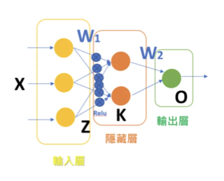
神經網路示意圖

假設

  • 輸入層有 3 個節點,輸入 X 中有 3 筆數據,其標籤為 Y:

X=[1202−32−1−13],Y=[12−3] X = \begin{bmatrix} 1 & 2 & 0 \\ 2 & -3 & 2 \\ -1 & -1 & 3 \\ \end{bmatrix}, Y = \begin{bmatrix} 1 \\ 2 \\ -3 \\ \end{bmatrix}

W1=[−10−111−1] W_1 = \begin{bmatrix} -1 & 0 \\ -1 & 1 \\ 1 & -1 \\ \end{bmatrix}

  • 隱藏層有 2 個節點,隱藏層權重矩陣為 W1W_1,線性組合 Z=XW1Z=XW_1,
    經過激活函數 σ\sigma 後的值為 KK,即 K=σ(Z)K = \sigma(Z)
  • 另激活函數 σ\sigma 為 ReluRelu 函數, σ(x)=Relu(x)=max(x,0)\sigma(x)=Relu(x)=max(x,0)
  • 輸出層有 1 個節點,其權重矩陣為 W2W_2,線性輸出 O=KW2O=KW_2

W2=[1−2] W_2 = \begin{bmatrix} 1 \\ -2 \\ \end{bmatrix}

  • 將輸出值與標籤去計算損失,令損失為 JJ,假設使用加總型式的最小平方損失

J=∑(12(O−Y)2)J = \sum (\frac{1}{2}(O-Y)^2)

此時,已知輸出層梯度:

Gout=∂J∂O=O−YG_{out} = \frac{\partial J}{\partial O}=O-Y

  • 隱藏層梯度:

G2=∂J∂W2=∂J∂O∂O∂W2=((Gout)T⋅K)T=KTGout\begin{equation} \begin{aligned} G_2 &= \frac{\partial J}{\partial W_2} = \frac{\partial J}{\partial O} \frac{\partial O}{\partial W_2} \\\\ &= ((G_{out})^T \cdot K)^T = K^TG_{out} \end{aligned} \end{equation}

  • ReluRelu 函數的微分式:

σ′(x)={0x<01x≥0\sigma^{\prime}(x) = \begin{cases} 0 \quad x < 0 \\ 1 \quad x \ge 0 \\ \end{cases}

  • 先假定一個暫存的 GtempG_{temp} :

Gtemp=(Gout⋅W2T)∘σ′(Z)G_{temp} = (G_{out} \cdot W^T_2) \circ \sigma^{\prime}(Z)

其中的 ⋅\cdot 代表一般的矩陣乘法、∘\circ 代表阿達瑪乘積,為對應位置的矩陣元素乘積

  • 輸入層梯度:

G1=∂J∂W1=∂J∂O∂O∂K∂K∂Z∂Z∂W1=(((Gout⋅W2T)∘σ′(Z))T⋅X)T=((Gtemp)T⋅X)T=XTGtemp\begin{equation} \begin{aligned} G_1 &= \frac{\partial J}{\partial W_1} = \frac{\partial J}{\partial O} \frac{\partial O}{\partial K} \frac{\partial K}{\partial Z} \frac{\partial Z}{\partial W_1} \\\\ &= (((G_{out} \cdot W^T_2) \circ \sigma^{\prime} (Z))^T \cdot X)^T \\\\ &= ((G_{temp})^T \cdot X)^T \\\\ &= X^TG_{temp} \end{aligned} \end{equation}

  • 可用 G1,G2G_1,G_2 梯度更新權重 W1,W2W_1,W_2 的值,得到新權重 W1new,W2newW_1^{new},W_2^{new},

假設我們採用隨機梯度下降法來進行更新,且學習率令為 0.10.1,則

{W1new=W1−0.1×G1W2new=W2−0.1×G2\begin{cases} W_1^{new} = W_1 - 0.1 \times G_1 \\ W_2^{new} = W_2 - 0.1 \times G_2 \\ \end{cases}

問題

求矩陣 Z,K,O,Gout,G2,σ′(Z),Gtemp,G1,W1new,W2newZ,K,O,G_{out},G_2,\sigma^{\prime}(Z),G_{temp},G_1,W_1^{new},W_2^{new}

求解過程皆省略公式推導過程,將直接使用最終結果代入計算


ZZ

由線性組合 Z=XW1Z=XW_1:

Z=XW1=[1202−32−1−13]⋅[−10−111−1]=[−323−55−4]\begin{equation} \begin{aligned} Z &= XW_1 \\\\ &= \begin{bmatrix} 1 & 2 & 0 \\ 2 & -3 & 2 \\ -1 & -1 & 3 \\ \end{bmatrix} \cdot \begin{bmatrix} -1 & 0 \\ -1 & 1 \\ 1 & -1 \\ \end{bmatrix} \\\\ &= \begin{bmatrix} -3 & 2 \\ 3 & -5 \\ 5 & -4 \\ \end{bmatrix} \end{aligned} \end{equation}


KK

由經過激活函數 σ\sigma 後的值 K=σ(Z)K = \sigma(Z),且激活函數 σ\sigma 為 ReluRelu 函數, σ(x)=Relu(x)=max(x,0)\sigma(x)=Relu(x)=max(x,0):

K=σ(Z)=σ ([−323−55−4])=[023050]\begin{equation} \begin{aligned} K &= \sigma(Z) \\\\ &= \sigma\ ( \begin{bmatrix} -3 & 2 \\ 3 & -5 \\ 5 & -4 \\ \end{bmatrix} ) \\\\ &= \begin{bmatrix} 0 & 2 \\ 3 & 0 \\ 5 & 0 \\ \end{bmatrix} \end{aligned} \end{equation}


OO

輸出層有 1 個節點,其權重矩陣為 W2W_2,由線性輸出 O=KW2O=KW_2:

O=KW2=[023050]⋅[1−2]=[−435]\begin{equation} \begin{aligned} O &= KW_2 \\\\ &= \begin{bmatrix} 0 & 2 \\ 3 & 0 \\ 5 & 0 \\ \end{bmatrix} \cdot \begin{bmatrix} 1 \\ -2 \\ \end{bmatrix} \\\\ &= \begin{bmatrix} -4 \\ 3 \\ 5 \\ \end{bmatrix} \end{aligned} \end{equation}


GoutG_{out}

由輸出層梯度 Gout=O−YG_{out} = O-Y:

Gout=O−Y=[−435]−[12−3]=[−518]\begin{equation} \begin{aligned} G_{out} &= O-Y \\\\ &= \begin{bmatrix} -4 \\ 3 \\ 5 \\ \end{bmatrix} - \begin{bmatrix} 1 \\ 2 \\ -3 \\ \end{bmatrix} \\\\ &= \begin{bmatrix} -5 \\ 1 \\ 8 \\ \end{bmatrix} \end{aligned} \end{equation}


G2G_2

由隱藏層梯度 G2=KTGoutG_2 = K^TG_{out},其中 KTK^T 為 矩陣 KK 的轉置:

K=[023050],KT=[035200]K = \begin{bmatrix} 0 & 2 \\ 3 & 0 \\ 5 & 0 \\ \end{bmatrix}, K^T = \begin{bmatrix} 0 & 3 & 5 \\ 2 & 0 & 0 \\ \end{bmatrix}

G2=KTGout=[035200]⋅[−518]=[43−10]\begin{equation} \begin{aligned} G_2 &= K^TG_{out} \\\\ &= \begin{bmatrix} 0 & 3 & 5 \\ 2 & 0 & 0 \\ \end{bmatrix} \cdot \begin{bmatrix} -5 \\ 1 \\ 8 \\ \end{bmatrix} \\\\ &= \begin{bmatrix} 43 \\ -10 \\ \end{bmatrix} \end{aligned} \end{equation}


σ′(Z)\sigma^{\prime}(Z)

其中 σ′\sigma^{\prime} 為 ReluRelu 函數的微分式:

σ′(x)={0x<01x≥0\sigma^{\prime}(x) = \begin{cases} 0 \quad x < 0 \\ 1 \quad x \ge 0 \\ \end{cases}

σ′(Z)=σ′([−323−55−4])=[011010]\begin{equation} \begin{aligned} \sigma^{\prime}(Z) &= \sigma^{\prime}( \begin{bmatrix} -3 & 2 \\ 3 & -5 \\ 5 & -4 \\ \end{bmatrix}) \\\\ &= \begin{bmatrix} 0 & 1 \\ 1 & 0 \\ 1 & 0 \\ \end{bmatrix} \end{aligned} \end{equation}


GtempG_{temp}

由假定暫存的 Gtemp=(Gout⋅W2T)∘σ′(Z)G_{temp} = (G_{out} \cdot W^T_2) \circ \sigma^{\prime}(Z)
其中的 ⋅\cdot 代表一般的矩陣乘法、∘\circ 代表阿達瑪乘積,為對應位置的矩陣元素乘積,且 W2TW_2^T 為矩陣 W2W_2 的轉置:

W2=[1−2],W2T=[1−2]W_2 = \begin{bmatrix} 1 \\ -2 \\ \end{bmatrix}, W_2^T = \begin{bmatrix} 1 & -2 \\ \end{bmatrix}

Gtemp=(Gout⋅W2T)∘σ′(Z)=([−518]⋅[1−2])∘[011010]=[−5101−28−16]∘[011010]=[0101080]\begin{equation} \begin{aligned} G_{temp} &= (G_{out} \cdot W^T_2) \circ \sigma^{\prime}(Z) \\\\ &= ( \begin{bmatrix} -5 \\ 1 \\ 8 \\ \end{bmatrix} \cdot \begin{bmatrix} 1 & -2 \end{bmatrix} ) \circ \begin{bmatrix} 0 & 1 \\ 1 & 0 \\ 1 & 0 \\ \end{bmatrix} \\\\ &= \begin{bmatrix} -5 & 10 \\ 1 & -2 \\ 8 & -16 \\ \end{bmatrix} \circ \begin{bmatrix} 0 & 1 \\ 1 & 0 \\ 1 & 0 \\ \end{bmatrix} \\\\ &= \begin{bmatrix} 0 & 10 \\ 1 & 0 \\ 8 & 0 \\ \end{bmatrix} \end{aligned} \end{equation}


G1G_1

由輸入層梯度 G1=XTGtempG_1 = X^TG_{temp},其中 XTX^T 為 矩陣 XX 的轉置:

X=[1202−32−1−13],XT=[12−12−3−1023],X = \begin{bmatrix} 1 & 2 & 0 \\ 2 & -3 & 2 \\ -1 & -1 & 3 \\ \end{bmatrix}, X^T = \begin{bmatrix} 1 & 2 & -1 \\ 2 & -3 & -1 \\ 0 & 2 & 3 \\ \end{bmatrix},

G1=XTGtemp=[12−12−3−1023]⋅[0101080]=[−610−1120260]\begin{equation} \begin{aligned} G_1 &= X^TG_{temp} \\\\ &= \begin{bmatrix} 1 & 2 & -1 \\ 2 & -3 & -1 \\ 0 & 2 & 3 \\ \end{bmatrix} \cdot \begin{bmatrix} 0 & 10 \\ 1 & 0 \\ 8 & 0 \\ \end{bmatrix} \\\\ &= \begin{bmatrix} -6 & 10 \\ -11 & 20 \\ 26 & 0 \\ \end{bmatrix} \end{aligned} \end{equation}


W1new,W2newW_1^{new},W_2^{new}

  • 可用 G1,G2G_1,G_2 梯度更新權重 W1,W2W_1,W_2 的值,得到新權重 W1new,W2newW_1^{new},W_2^{new},
    已知我們採用隨機梯度下降法來進行更新,且學習率為 0.10.1,則

{W1new=W1−0.1×G1W2new=W2−0.1×G2\begin{cases} W_1^{new} = W_1 - 0.1 \times G_1 \\ W_2^{new} = W_2 - 0.1 \times G_2 \\ \end{cases}

W1new=W1−0.1×G1=[−10−111−1]−0.1×[−610−1120260]=[−10−111−1]−[−0.61−1.122.60]=[−0.4−10.1−1−1.6−1]\begin{equation} \begin{aligned} W_1^{new} &= W_1 - 0.1 \times G_1 \\\\ &= \begin{bmatrix} -1 & 0 \\ -1 & 1 \\ 1 & -1 \\ \end{bmatrix} - 0.1 \times \begin{bmatrix} -6 & 10 \\ -11 & 20 \\ 26 & 0 \\ \end{bmatrix} \\\\ &= \begin{bmatrix} -1 & 0 \\ -1 & 1 \\ 1 & -1 \\ \end{bmatrix} - \begin{bmatrix} -0.6 & 1 \\ -1.1 & 2 \\ 2.6 & 0 \\ \end{bmatrix} \\\\ &= \begin{bmatrix} -0.4 & -1 \\ 0.1 & -1 \\ -1.6 & -1 \\ \end{bmatrix} \end{aligned} \end{equation}

W2new=W2−0.1×G2=[1−2]−0.1×[43−10]=[−10−111−1]−[4.3−1]=[−3.3−1]\begin{equation} \begin{aligned} W_2^{new} &= W_2 - 0.1 \times G_2 \\\\ &= \begin{bmatrix} 1 \\ -2 \\ \end{bmatrix} - 0.1 \times \begin{bmatrix} 43 \\ -10 \\ \end{bmatrix} \\\\ &= \begin{bmatrix} -1 & 0 \\ -1 & 1 \\ 1 & -1 \\ \end{bmatrix} - \begin{bmatrix} 4.3 \\ -1 \\ \end{bmatrix} \\\\ &= \begin{bmatrix} -3.3 \\ -1 \\ \end{bmatrix} \end{aligned} \end{equation}


回到導覽頁面